Classification Analysis: Predicting the Gender of Bikeshare Users
The full code can be found here.
Bike-sharing services offer a means for people to quickly access affordable, short term transportation in urban areas. Increased automation has allowed for these services to grow more robust in nature and generate more data. Such data can be used to make improvements in area such as product development and marketing. By being able to get a comprehensive picture of the people using bike share services, changes can be made that could directly benefit the users of the service. Such efficient decisionmaking can generate growth and increase revenue for bike-sharing companies. For this reason, I am interested in predicting the gender of NYC Citi Bike users by creating a model based on the data generated from the service.
The Citi Bike service works by allowing people to pick up bikes at one of hundreds of stations in Manhattan, Brooklyn, Queens and Jersey City. The users can ride for a predetermined amount of time based on the passes or memberships that they purchase. They end their time with the bikes by returning them to any of the affiliated stations.
In this study, several types of supervised learning classification models were used to predict the gender of the Citi Bike Users. Models focused on utilizing factors related to the individual uses of the service. The different models were compared to better understand their ability to accurately predict gender using multiple forms of statistical evaluation. The process used to undertake the study is as follows:
Data Exploration and Analysis
- Viewing the Distribution of the Different Classes
- Checking the Correlatedness of Different Variables
- Interpreting Descriptive Statistics
Preparing The Data For Modeling
- Imputing Outliers
- Class Balancing
- Feature Selection
Modeling the Data
- Using All Useful Features
- Using PCA Components
- Using Selectkbest Function
Data Exploration and Analysis
The Citi Bike Trip Dataset contains information about 735502 anonymised trips that took place between January 2015 and June 2017. The data was processed to remove trips that are taken by staff and any trips that were below 60 seconds in length. The dataset originally contained columns related to the location of the stations, duration of the trips, and demographics of the users. Additional features were engineered with this information such as the distance between the stations used in a trip and the age of the users.
| start_station_id | start_station_name | start_station_latitude | start_station_longitude | end_station_id | end_station_name | end_station_latitude | end_station_longitude | trip_duration | start_time | stop_time | bike_id | user_type | birth_year | gender | |
|---|---|---|---|---|---|---|---|---|---|---|---|---|---|---|---|
| 0 | 3212 | Christ Hospital | 40.735 | -74.050 | 3207 | Oakland Ave | 40.738 | -74.052 | 376 | 2015-10-01 00:16:26 | 2015-10-01 00:22:42 | 3212 | Subscriber | 1960.000 | 1 |
| 1 | 3207 | Oakland Ave | 40.738 | -74.052 | 3212 | Christ Hospital | 40.735 | -74.050 | 739 | 2015-10-01 00:27:12 | 2015-10-01 00:39:32 | 3207 | Subscriber | 1960.000 | 1 |
| 2 | 3193 | Lincoln Park | 40.725 | -74.078 | 3193 | Lincoln Park | 40.725 | -74.078 | 2714 | 2015-10-01 00:32:46 | 2015-10-01 01:18:01 | 3193 | Subscriber | 1983.000 | 1 |
| 3 | 3199 | Newport Pkwy | 40.729 | -74.032 | 3187 | Warren St | 40.721 | -74.038 | 275 | 2015-10-01 00:34:31 | 2015-10-01 00:39:06 | 3199 | Subscriber | 1975.000 | 1 |

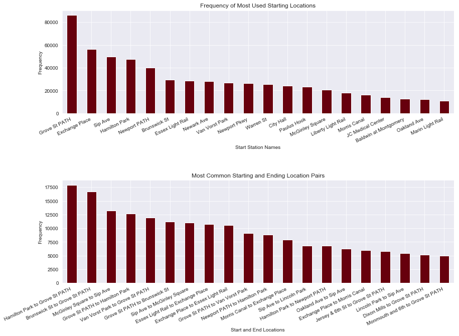
The bar graphs above references the number of trips that took place over the two year perion during which the data was collected and only represents the classes with the highest frequencies. While the station names aren’t going to be useful to for modeling due to the high number of classes relative to the number of observations, it’s useful for gaining an understanding of the nature in which the service is used.

The distribution of the frequency of distances between the start and end stations center around 1 km and the majority of trips lasted less than 10 minutes. It is important to note that while trip duration and distance are correlated, the users aren’t necessarily riding the bikes during the entire time period in which the bikes are checked out.

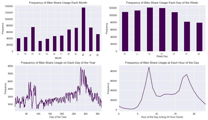
Most of the trips took place during the Fall with October experiencing a disproportionately higher use of the Citi Bike service. The frequency of Citi Bike trips was consistent during the weekday and dropped during weekends. With regards to the time of day, most trips took place during the morning and evening. These trends correspond to the average American work week.
The vast majority of the services users are subscribers (annual membership holders) as opposed to customers (single day or 3-day pass holders. While there is a sharp difference between rates of the two user types the model may be able to capture subtle differences between the types of users that could aid in prediction.
1    525608
2    150426
0     59468
Name: gender, dtype: int64
The 1 class refers to the number of trips that were taken by a male and the 2 class refers to the number of trips that were taken by a female. The the gender is unknown for the observations that contain a 0 gender class. The sharp imbalance in the gender class will need to be remedied prior to modeling. The 0 class observations will need to be discarded prior to modeling but even without them, there are enough observations to make a large enough sample of the original dataset.

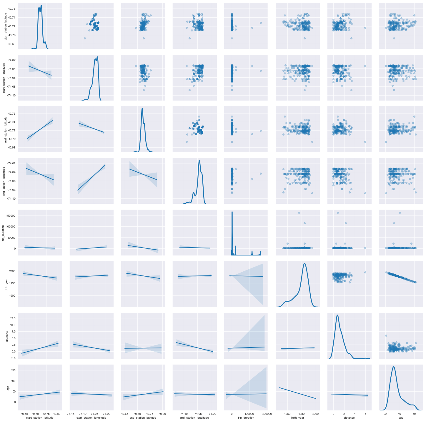
This scatterplot matrix was made to analyze the relationship between the continuous variables. The topright half of the matrix gives scatterplots of each combination of variables while the bottom left gives the best fit lines corresponding to the relationship between each pair. The diagonals consist of KDE plots which show the shape of the distribution of each variable.

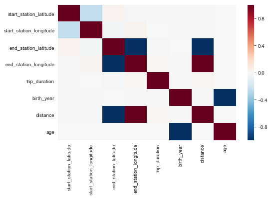
Aside from the variables directly related to the locations of the stations, most of the features of this dataset have little to no correlation.
| start_station_latitude | start_station_longitude | end_station_latitude | end_station_longitude | trip_duration | birth_year | gender | distance | month | start_day_of_week_number | start_day_of_month | start_day_of_year | start_hour | start_timestamp | age | |
|---|---|---|---|---|---|---|---|---|---|---|---|---|---|---|---|
| count | 735502.000 | 735502.000 | 735502.000 | 735502.000 | 735502.000 | 735502.000 | 735502.000 | 735502.000 | 735502.000 | 735502.000 | 735502.000 | 735502.000 | 735502.000 | 735502.000 | 735502.000 |
| mean | 40.723 | -74.046 | 40.722 | -74.045 | 934.312 | 1979.544 | 1.124 | 1.148 | 7.264 | 2.779 | 15.748 | 206.134 | 13.599 | 1467895633.510 | 36.408 |
| std | 0.008 | 0.011 | 0.095 | 0.173 | 40638.782 | 9.371 | 0.520 | 19.717 | 3.372 | 1.909 | 8.775 | 102.695 | 5.226 | 13579046.873 | 9.382 |
| min | 40.693 | -74.097 | 0.000 | -74.097 | 61.000 | 1900.000 | 0.000 | 0.000 | 1.000 | 0.000 | 1.000 | 1.000 | 0.000 | 1442847196.000 | 16.000 |
| 25% | 40.718 | -74.051 | 40.717 | -74.050 | 246.000 | 1975.000 | 1.000 | 0.621 | 4.000 | 1.000 | 8.000 | 114.000 | 9.000 | 1458289118.500 | 30.000 |
| 50% | 40.722 | -74.044 | 40.721 | -74.044 | 383.000 | 1982.000 | 1.000 | 0.883 | 8.000 | 3.000 | 16.000 | 231.000 | 14.000 | 1470155248.000 | 34.000 |
| 75% | 40.728 | -74.038 | 40.727 | -74.036 | 652.000 | 1986.000 | 1.000 | 1.467 | 10.000 | 4.000 | 23.000 | 292.000 | 18.000 | 1477541380.000 | 41.000 |
| max | 40.753 | -74.032 | 40.801 | 0.000 | 20260211.000 | 2000.000 | 2.000 | 8449.122 | 12.000 | 6.000 | 31.000 | 366.000 | 23.000 | 1491002734.000 | 116.000 |
These descriptive statistics supplement the scatterplot matrix by quantifying the distribution of the variables. The distributions of the variables related to location and time are relatively consistent because they a limited range and fixed frequencies (e.g. the max start_day_of_month would be 31 because that’s the maximum number of days in a month). Potential outliers do exist in the variables that aren’t limited to a specific range such as, trip_duration, diatance, and age.

These boxplots show that there are outliers in the features that are not fixed to a specific range. Take note of the logarithmic scale being used for trip_duration and distance. This means that any gaps in the points shown for those two plots represent a large amount of distance between the actual points.
Preparing The Data For Modeling
To prepare the data for modeling, features were selected, the data was resampled to address the class imbalance in the outcome, and three forms of feature selection were implemented. This resulted in three sets of variables: One reflecting all of the useful features of the dataset, one reflecting PCA components, and one reflecting features chosen by the selectKbest function.
Features that were useful for modeling were isolated into a final dataframe that would be used for training and testing along side versions of the dataframe that underwent different forms of feature selection.
%%time

## Train Test Split the Three Sets of Feature and Outcome Variables

x_train, x_test, y_train, y_test = train_test_split(x, y, test_size=0.2, random_state=20)

kx_train, kx_test, ky_train, ky_test = train_test_split(k_predictors, y, test_size=0.2, random_state=21)

px_train, px_test, py_train, py_test = train_test_split(pca_components, y, test_size=0.2, random_state=22)
Training and testing sets of three variables were generated to be used in modeling. The x and y variables represent the variables to be used for modeling that reflect the all of the useful features of the data. The px and py variables represent the variables to be used for modeling that reflect PCA components of the initial features. The kx and ky variables represent the variables to be used for modeling that reflect features chosen by selectKbest.
Modeling the Data using all Useful Features
Random Forest
accuracy score:
0.9426571428571429

cross validation:
[0.811942   0.82264286 0.82185714 0.81464286 0.8173441 ]

cross validation with AUC:
[0.90020833 0.90318671 0.89839968 0.89670665 0.90036234]

confusion matrix:
[[32719  2417]
 [ 1597 33267]]

              precision    recall  f1-score   support

           1       0.95      0.93      0.94     35136
           2       0.93      0.95      0.94     34864

   micro avg       0.94      0.94      0.94     70000
   macro avg       0.94      0.94      0.94     70000
weighted avg       0.94      0.94      0.94     70000
The random forest model had the best performance out of all of the models run with all of the dataset’s useful features. Cross validation showed few signs of overfitting with this model. The strength of this model when it comes to making predictions using this data comes from its ability to separate datapoints using binary splits, which is especially useful for isolated latitude and longitude features. The decision tree had similar accuracy scores but lower cross validation scores. Naive bayes performed poorly with this data. This is likely due to the naturally high correlatedness of variables related to station locations. The support vector classifier didn’t have the best performance but there is room for this model to improve as computational resources increase in availability. KNN and logistic regression had poor performance (although better than Naive Bayes). This likely has to do with these models being unable to capture nuances between different groups of observations and the interactions between the variables.
In general, the models that relied on the dataset’s most useful features had the best performance in the study. An advantage of using all of the useful features is that as much meaningful variance was captured by the models as possible. This method of feature selection also risks including features with variance that doesn’t aid in the predictive power of the models. However, this potential disadvantage didn’t hamper the model’s ability to perform well because many of the features that would noticeably have a negative effect on the models were already left out.
Modeling the Data using PCA Components
Random Forest
accuracy score:
0.9099

cross validation:
[0.7205     0.71721429 0.72242857 0.718      0.71907143]

cross validation with AUC:
[0.79895943 0.79188841 0.79536728 0.79454343 0.79382654]

confusion matrix:
[[31428  3557]
 [ 2750 32265]]

              precision    recall  f1-score   support

           1       0.92      0.90      0.91     34985
           2       0.90      0.92      0.91     35015

   micro avg       0.91      0.91      0.91     70000
   macro avg       0.91      0.91      0.91     70000
weighted avg       0.91      0.91      0.91     70000
The random forest model had the best performance out of all of the models run with 15 of the dataset’s best PCA components. While cross validation did show few signs of overfitting with this model, those scores were significantly lower than the accuracy score. This is a noticeably lower performance than the random forest model that used all of the available features. In general, the models that used the PCA components had lower scores than the models that used all of the dataset’s useful features and the models that used features chosen by selectKbest. However, KNN and naive bayes did perform better with PCA components. The increase in performance of these two model types can be attributed to the increased significance of the remaining components allowing the algorithms to better classify the observations.
Using a limited number of PCA components from the dataset likely removed some variance that was important to the predictive accuracy of the models. Using PCA components does have the advantage of reducing computational complexity and runtimes but this did not make up for the drop in accuracy of the better performing model types.
Modeling the Data using Features Chosen with the SelectKbest Function
Random Forest
accuracy score:
0.9357

cross validation:
[0.82772659 0.82151275 0.8145     0.81962997 0.81605829]

cross validation with AUC:
[0.89991833 0.9033447  0.90034001 0.89884141 0.90075802]

confusion matrix:
[[32054  2789]
 [ 1712 33445]]

              precision    recall  f1-score   support

           1       0.95      0.92      0.93     34843
           2       0.92      0.95      0.94     35157

   micro avg       0.94      0.94      0.94     70000
   macro avg       0.94      0.94      0.94     70000
weighted avg       0.94      0.94      0.94     70000

CPU times: user 25min 54s, sys: 33.1 s, total: 26min 27s
Wall time: 26min 36s
The random forest model had the best performance out of all of the models run with features chosen using the selectkbest function. Cross validation showed few signs of overfitting with this model. The random forest model using selectkbest still had lower accuracy than the model that used all of the available features in the dataset, implying that useful features were removed prior to modeling. Since selectKbest removes a low number of features in this case, this would mean that the majority of the dataset’s useful features had meaningful variance . Logistic regression’s performance didn’t differ much regardless of feature selection, implying that the model type doesn’t suit the bikeshare data.
When it comes to comparing full featured models and models that used sectkbest, most of the full featured models slightly outperformed their counterparts that used K best features. Using selectKbest allows for computational complexity to be reduced without abstracting the individual features (unlike PCA). However, in a situation where most of the features had a positive effect on the ability of the model to predict gender, this form of feature selection wasn’t particularly helpful.
Analysis and Conclusion
The random forest model using all of the dataset’s useful features the best model when it came to predicting the gender of the Citi Bike users. It is also important to note that the support vector classifier could also prove valuable when it comes to making predictions if larger amounts of computational resources are available due to its ability to draw distinct boundaries among the classes; a quality that is especially useful for location based data.
This study established the best suprvised modeling technique and feature classification pairing for the gender of the citibike users. The next step in using this data to discern the demographics of the users based on their usage of the service would be to collect more types of data and go more in depth into which features have a greater impact on the likelihood of a user being a particular gender. This includes collecting data from different sources and engineering more features. Afterwards the study can be expanded to include different types of demographical classes as outcomes such as age.
Understanding how to better utilize supervised modeling techniques to predict gender, will give insight as to what kind of people are using the bike share service and particular habits different types of customers share. This can allow for more direct marketing to specific types of users or changes in the product that better match how the service is used. Through the use of cheap and accessible data, decisions can be made that can result in increased efficiency and revenue for the company.

