Regression Analysis: Predicting Ames Housing Market Prices
The full code can be found here.
Housing prices have steadily increased over the course of the past three decades with the exception of severe economic downturns such as the economic recession of 2008. The housing market is not only a very strong economic indicator but it has a financial impact on anyone looking to own a home themselves. To better understand the effects that individual factors have on the housing prices, I am interested in using supervised learning techniques to model housing prices. By using machine learning techniques to do this the process can be automated to include a large amount of data points and different trends can be detected that may not be readily apparent to humans.
In this study, several types of supervised learning classification models were used to predict housing prices in Ames, Iowa. Models focused on utilizing multiple housing price indicators, including factors related to the size and location of the living spaces. The different models were compared to better understand their ability to utilize the data to accurately predict the housing market using multiple forms of statistical evaluation. The process used to undertake this study is as follows:
Initiation and Data Preprocessing
- Importing Packages and Files
- Defining Reusable Functions
- Data Exploration and Cleaning
Exploratory Data Analysis
- Identifying Statistically Significant Features
- Univariate, Bivariate, and Multivariate Analysis
- Analyzing the Relationship Between the Variables
- Descriptive Statistics and Boxplots
Predictive Modeling and Evaluation
- Data Preprocessing
- Lasso Regression
- Elastic Net Regression
- Random Forests
- Gradient Boost
- Creating Price Predictions
Exploratory Data Analysis
Dataset used for this study includes information about home purchases in Ames pertaining to their physical qualities and how they were sold. Such information includes: the location of the homes, the spatial dimensions of the homes, and the methods in which the homes were sold.
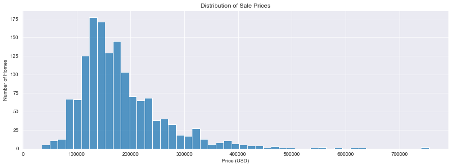
The mean sale price is $180,921 and the median sale price is $163,000. The distribution of the sale prices is skewed to the right. A logarithmic transformation can be used to make the sale prices more normally distributed prior to modeling.
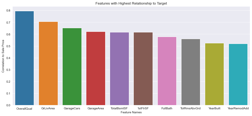
The above plot displays the ten continuous features with the highest linear relationship to the sales price. The units used to describe this is the absolute value of the correlation coefficient (range 0 to 1). Variables with a correlation coefficient of .5 or higher have a strong linear relationship with the sales price (variables with lower correlation coefficients are not shown here).
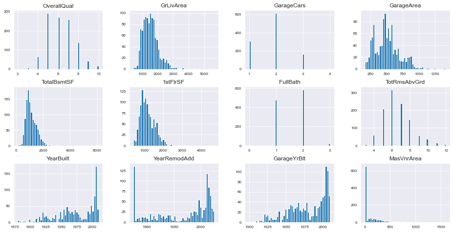
The above histograms display the distribution of the top features. The histograms are ordered based on the features’ correlation to the sale price (most correlated to least correlated). As the correlation decreases, the distribution of the features have less of a resemblance to the distribution of the sale price.
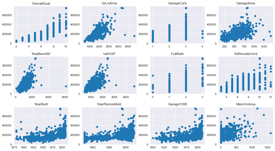
The above scatterplots display the relationship of the top features to the sale price. The scatterplots are ordered based on the features’ correlation to the sale price (most correlated to least correlated). As the correlation decreases, features display less of a linear relationship with sales price.
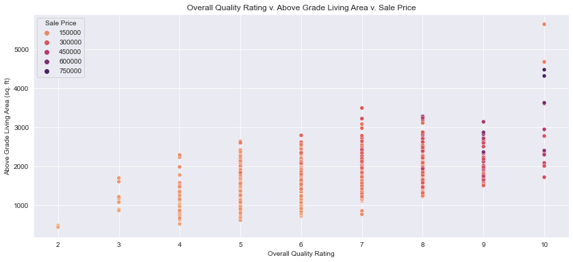
With the exception of a couple of outliers, quality rating and above grade living area when paired together have a strong linear relationship with sale price.
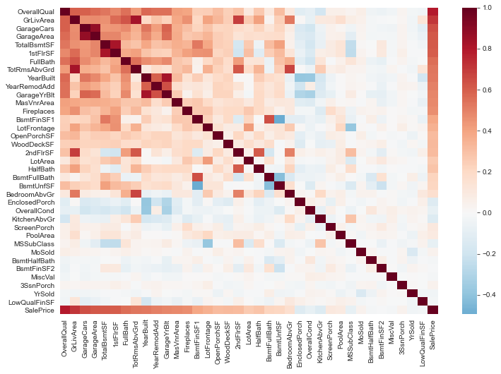
There are strong correlations among features that measure a similar quality of the homes (such as the year the house was built and year the garage was built).
| count | mean | std | min | 25% | 50% | 75% | max | |
|---|---|---|---|---|---|---|---|---|
| OverallQual | 1094.0 | 6.247715 | 1.366797 | 2.0 | 5.0 | 6.0 | 7.0 | 10.0 |
| GrLivArea | 1094.0 | 1535.027422 | 526.124028 | 438.0 | 1164.0 | 1480.0 | 1779.0 | 5642.0 |
| GarageCars | 1094.0 | 1.879342 | 0.658586 | 1.0 | 1.0 | 2.0 | 2.0 | 4.0 |
| GarageArea | 1094.0 | 503.760512 | 192.261314 | 160.0 | 360.0 | 484.0 | 602.5 | 1418.0 |
| TotalBsmtSF | 1094.0 | 1099.561243 | 415.851262 | 105.0 | 816.0 | 1023.0 | 1345.5 | 6110.0 |
| 1stFlrSF | 1094.0 | 1173.809872 | 387.677463 | 438.0 | 894.0 | 1097.0 | 1413.5 | 4692.0 |
| SalePrice | 1094.0 | 187033.263254 | 83165.332151 | 35311.0 | 132500.0 | 165750.0 | 221000.0 | 755000.0 |
Due to the presence of outliers, the median (the column denoted ‘50%’) displays information that is more representative of the data.
Predictive Modeling and Evaluation
Models are evaluated by using the following metrics on the validation set: R-squared value, root mean square error, and mean absolute error. Additionally, the residuals from the validation set are plotted and analyzed.
Gradient Boost
Validation Set Evaluation

R squared score:
0.9172114815362296

RMSE: 22058.97119044775

MAE: 14769.614705646483
The gradient boost model had the best performance out of all of the models. Cross validation showed fewer signs of overfitting with this model. The strength of this model when it comes to making predictions using this data comes from its ability to reduce error over multiple iterations, resulting in higher accuracy scores after a high number of iterations.
Creating Price Predictions For Unsold Homes
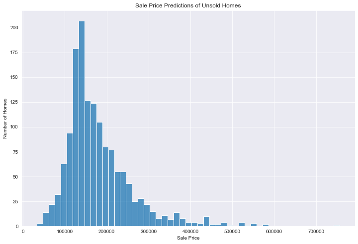
The gradient boosting model was used to predict the sale prices of unsold homes. The predicted sale prices, have a similar distribution to the known sale prices. Most of the homes that have yet to be sold will likely be sold for around $150,000.
Final Analysis and Conclusion
Understanding how to better utilize supervised modeling techniques to predict housing prices will give insight into which factors have the most effect on the prices of homes. Information about how such trends change over time can also be gained, which will be useful in understanding the real estate market which is a major economic indicator.
This study established the best suprvised modeling technique for predicting housing prices. The next step in using this data to gather insights from sales of homes would be to collect housing data from greater time spans (involving similar homes) and use them to train a model that will focus on seasonality and change over time. By being able to understand how such supervised learning models can be improved with the added context of time, housing prices can be predicted even more accurately and more information can be gained about the housing market that can provide actionable insights.

