

Comprehensive Modeling Analysis: Predicting Airbnb New User Bookings
The full code can be found here.
Home rental services such as Airbnb allow people to find affordable temporary housing on short notice. The efficiency of these services can be increased by making decisions informed by knowledge about how future customers will use them. By being able to determine how new customers will use home rental services for the first time, proactive changes can be made to the service and the surrounding operations. This results in a better product for the customers and improved operations for stakeholders. Data science techniques allow for the prediction of future user activities at the cost of relatively few resources. The abundance of data generated by short-term home rental services such as Airbnb, allows for plenty of opportunities for data science to be used to improve the operations. In order to utilize this readily usable data, I am interested in predicting booking destinations of first time Airbnb users.
Airbnb’s platform allows customers to efficiently find homes that fit their needs through the use of features such as filtered searches and wishlists. After finding desirable lodging, customers input payment information and book the locations. Throughout this process data is generated through information provided by the users and details saved about the user’s web sessions.
Several types of classification models were used to predict the first booking destination countries of Airbnb users. Models focused on using demographic and web session data to assign booking destination countries to individual users. The different models were compared by their ability to accurately and efficiently predict booking country. A final model was chosen from those that were evaluated and deemed suitable to be scaled for production. The process used to build this product is as follows:
Initiation and Data Preprocessing
- Import Packages and Files
- Data Cleaning
- Feature Engineering
Data Analysis and Exploration
- Viewing the Distribution of the Different Classes
- Checking the Correlatedness of Different Variables
- Interpreting Descriptive Statistics
Preparing The Data For Modeling
- Class Balancing and Mathematical Transformations
- Feature Selection and Reduction
- Establishing Variables for Training and Testing
Supervised Learning Models
- Using Unaltered Features
- Using Features Selected using F Values
- Using Features Selected using Chi Squared
- Using Recurrent Neural Network
- Using Features Selected using Random Forests
Analysis and Conclusion
- Final Model Selection and Analysis
- Conclusion and Discussion
The purpose of this study is to: analyze user demographics and behavioral patterns via data visualization, identify key indicators of future behavior by utilizing statistical inference and machine learning algorithms, create a machine learning model that can predict the booking destination of users that haven’t made a booking yet, and use the aforementioned model to predict the future behavior of users that are currently on the platform.
Initiation and Data Preprocessing
The data used for this model was released by Airbnb in the following datasets: train_users.csv and sessions.csv. The train user dataset contains information about specific users and how they first accessed the service. This dataset has over 200000 records with each one containing information about a unique user. The train user dataset contains the outcome variable, country destination. The sessions dataset contains information about actions performed during the user’s time on the Airbnb platform. This dataset contains over 10 million records with each one reflecting a specific action performed on the platform. Multiple records on the sessions dataset can refer a single user’s actions. A dataframe was created for modeling containing features generated from both datasets.
Data Exploration and Analysis
The Airbnb data contains information about activity on the platform that occurred between January 2010 and June 2014. The train dataset originally contained columns related to the time specific activities first occured, information about the how the user accessed Airbnb, and demographics of the users. Additional features were engineered to include the amount of time users spent doing specific activities on the platform.
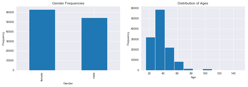
Above are plots representing the gender frequencies and age frequencies of the data, respectively. There are more females than males included in the data but the disparity between the two groups is not strong. The distribution of the ages is centered around the 30’s and skewed to the right. This likely reflects an age demographic with both the energy and resources to travel. Since both of these variables contain a large amount of null values imputation will be needed to make use of this data prior to modeling.
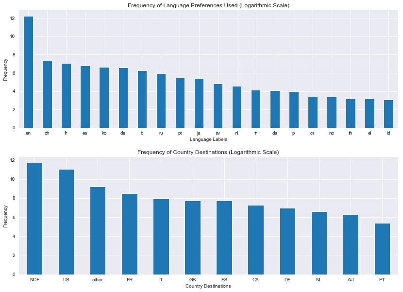
Above are plots of languages used on the platform and country destination, respectively. Both plots are scaled logarithmically for readability because the dominant classes far outnumbered the rest. With regard to the language counts, English outnumbered the other classes greatly; and with regard to the country destinations, ‘NDF’ and the US outnumbered the other classes. NDF represents the class of users that haven’t booked a destination yet. Since this would be the class that the model being built would be predicting, this was not be used as an outcome variable to train the model.
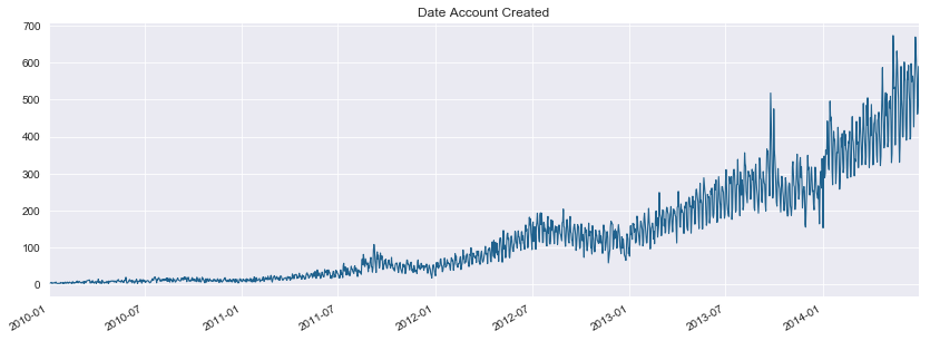
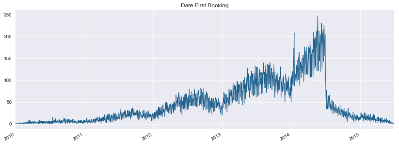
The above plots refer to the frequencies the accounts were first created and frequencies bookings were made over the course of multiple years. The frequency of accounts being created showed an increasing trajectory over the course of five years, likely reflecting an increase in the userbase of Airbnb. There is a sharp drop in bookings made around the time that the data was collected. This doesn’t reflect a drop in the usage of the platform, but rather people who use the platform but haven’t made a booking yet (these customers would have the country destination label ‘NDF’).
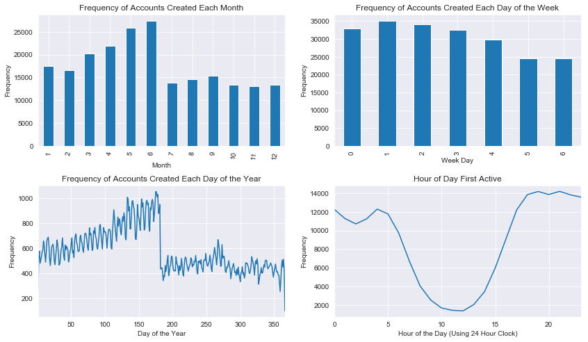
The above plots reflect the frequencies use of the platform created across different timespans. There’s a notable drop of accounts created between June and July. Since summer is a season that is popular for travel, people are less likely to need accounts during this time (because they would’ve presumably made accounts earlier than when they would travel using the service). There is a slight drop of accounts made over the weekends as well. Initial activity drops during the day which is likely the result of people having less time during the average US workday to be on Airbnb.
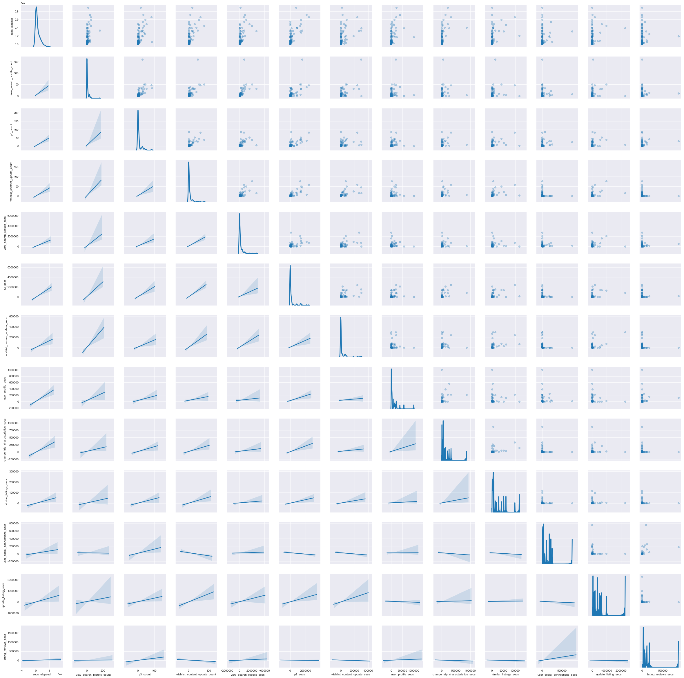
The scatterplot matrix gives information about the relationship between specific engineered features.
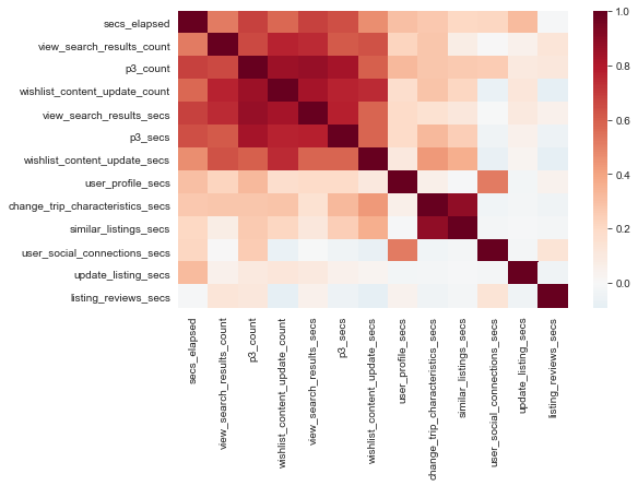
The heatmap is meant to gauge the correlatedness of engineered features. There is much correlatedness among these features, which is expected since they reflect amounts of time spent on the platform.
| secs_elapsed | view_search_results_count | p3_count | wishlist_content_update_count | user_profile_count | change_trip_characteristics_count | similar_listings_count | user_social_connections_count | update_listing_count | listing_reviews_count | ... | dashboard_secs | user_wishlists_secs | header_userpic_secs | message_thread_secs | edit_profile_secs | message_post_secs | contact_host_secs | unavailable_dates_secs | confirm_email_link_secs | create_user_secs | |
|---|---|---|---|---|---|---|---|---|---|---|---|---|---|---|---|---|---|---|---|---|---|
| count | 73815.000 | 73815.000 | 73815.000 | 73815.000 | 73815.000 | 73815.000 | 73815.000 | 73815.000 | 73815.000 | 73815.000 | ... | 73815.000 | 73815.000 | 73815.000 | 73815.000 | 73815.000 | 73815.000 | 73815.000 | 73815.000 | 73815.000 | 73815.000 |
| mean | 1514234.959 | 12.366 | 8.265 | 6.093 | 3.634 | 4.278 | 4.172 | 1.940 | 2.105 | 1.128 | ... | 14830.135 | 29595.309 | 4515.531 | 51134.615 | 16820.605 | 74545.834 | 21243.895 | 7023.293 | 94984.878 | 100.872 |
| std | 1913191.475 | 28.446 | 20.404 | 13.310 | 14.324 | 9.715 | 10.018 | 9.129 | 8.068 | 5.697 | ... | 112658.964 | 177757.650 | 45779.443 | 306877.869 | 93129.557 | 268323.753 | 104188.163 | 53648.290 | 259453.037 | 7967.568 |
| min | 0.000 | 0.000 | 0.000 | 0.000 | 0.000 | 0.000 | 0.000 | 0.000 | 0.000 | 0.000 | ... | 0.000 | 0.000 | 0.000 | 0.000 | 0.000 | 0.000 | 0.000 | 0.000 | 0.000 | 0.000 |
| 25% | 256920.500 | 0.000 | 0.000 | 0.000 | 0.000 | 0.000 | 0.000 | 0.000 | 0.000 | 0.000 | ... | 0.000 | 0.000 | 143.000 | 0.000 | 0.000 | 0.000 | 0.000 | 0.000 | 0.000 | 0.000 |
| 50% | 872862.000 | 2.000 | 2.000 | 1.000 | 0.000 | 0.000 | 0.000 | 0.000 | 0.000 | 0.000 | ... | 0.000 | 0.000 | 695.000 | 0.000 | 0.000 | 0.000 | 0.000 | 0.000 | 0.000 | 0.000 |
| 75% | 2043487.500 | 13.000 | 9.000 | 6.000 | 2.000 | 4.000 | 4.000 | 0.000 | 1.000 | 0.000 | ... | 1268.000 | 0.000 | 2356.000 | 0.000 | 0.000 | 1583.000 | 427.000 | 0.000 | 44589.000 | 0.000 |
| max | 38221363.000 | 987.000 | 1131.000 | 524.000 | 454.000 | 308.000 | 325.000 | 280.000 | 249.000 | 198.000 | ... | 4632786.000 | 6713259.000 | 2288760.000 | 11242289.000 | 3415239.000 | 13260005.000 | 3258808.000 | 2310246.000 | 2902601.000 | 1723704.000 |
8 rows × 39 columns
Data will be normalized prior to modeling to account for the vast difference in scale of the variables.
Preparing The Data For Modeling
To prepare the data for modeling, values were imputed, the data was resampled to address the class imbalance in the outcome, and multiple forms of feature reduction were implemented. This resulted in four sets of variables: One reflecting all of the unaltered features of the dataset, one reflecting features with the highest F values, one reflecting features with the highest chi squared values, and encoded for deep learning.
%%time

## Train Test Split the Four Sets of Feature and Outcome Variables

# Unaltered Features
x_train, x_test, y_train, y_test = train_test_split(pca_components, y, test_size=0.2, random_state=20)

# F-Value
fx_train, fx_test, fy_train, fy_test = train_test_split(f_pca_components, y, test_size=0.2, random_state=22)

# Chi-squared
xx_train, xx_test, xy_train, xy_test = train_test_split(x_pca_components, y, test_size=0.2, random_state=21)

# Deep Learning
X_train, X_test, Y_train, Y_test = train_test_split(np.asarray(f_pca_components), np.asarray(Y), test_size=0.2, random_state=20)
Modeling the Data using Features Chosen with Random Forests
Random Forest
Test Set Evaluation

accuracy score:
0.978989898989899

confusion matrix:
[[1782    0    0    0    0    0    0    0    0    0    0]
 [   0 1702    0    0    0    0    0    0    0    0    0]
 [   0    0 1840    0    0    0    0    0    0    0    0]
 [   0    0    0 1858    0    0    0    0    0    0    0]
 [   0    0    0    0 1747    0    0    0    0   12    2]
 [   0    0    0    0    0 1749    0    0    0    0    0]
 [   0    0    0    0    0    0 1801    0    0    0    0]
 [   0    0    0    0    0    0    0 1840    0    0    0]
 [   0    0    0    0    0    0    0    0 1808    0    0]
 [   1    4    2   10   50    8    9    2    0 1630  140]
 [   0    3    0    1    6    0    1    0    0  165 1627]]

              precision    recall  f1-score   support

          AU       1.00      1.00      1.00      1782
          CA       1.00      1.00      1.00      1702
          DE       1.00      1.00      1.00      1840
          ES       0.99      1.00      1.00      1858
          FR       0.97      0.99      0.98      1761
          GB       1.00      1.00      1.00      1749
          IT       0.99      1.00      1.00      1801
          NL       1.00      1.00      1.00      1840
          PT       1.00      1.00      1.00      1808
          US       0.90      0.88      0.89      1856
       other       0.92      0.90      0.91      1803

    accuracy                           0.98     19800
   macro avg       0.98      0.98      0.98     19800
weighted avg       0.98      0.98      0.98     19800
The model that relied on features selected using random forests had the best accuracy in the study (with a 97% test set accuracy). An advantage of using all of the useful features is that as much meaningful variance was captured by the models as possible. A downside to this type of feature preparation that did stand out is the lack of efficiency. Since feature reduction didn’t take place with these models, their performance suffered and they had the longest runtimes. However, for reporting purposes, accuracy was prioritized. This method of feature selection also risks including features with variance that doesn’t aid in the predictive power of the models. However, this potential disadvantage didn’t hamper the model’s ability to perform well because many of the features that would noticeably have a negative effect on the models were already left out.
Identifying the Most Important Features
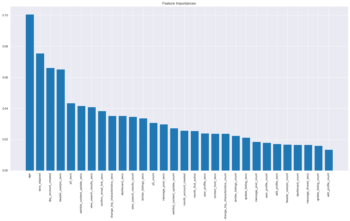
The above graph displays factors that contributed the most to the highly accurate predictions of booking destination. The age and the amount of time spent on the platform were the most useful factors in determining where a person was likely to book their next stay.
Generating Predictions of Current Users’ Booking Destinations
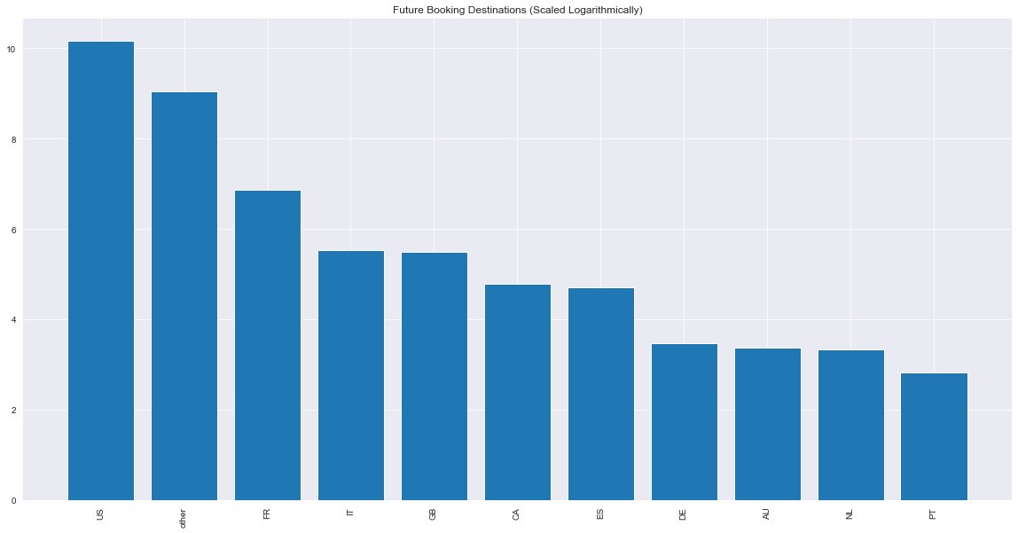
By using the most successful modeling type on the data of the users that haven’t booked housing with the platform, future usage of the Airbnb platform can be predicted and analyzed. The distribution of the plot above shows that France is the most likely destination for non-US Airbnb users.
Analysis and Conclusion
The random forest model using features chosen based on random forest feature importances was the best model when it came to predicting the first booking destinations, making it the strongest base for a classifier that can scaled for production. It was able to predict the booking destination of users with a 97% accuracy. While other model types had potential to produce more accurate predictions, they had much higher runtimes, making them unfit to run larger amounts of data. By introducing more data to this modeling pipeline, it can be trained to yield even more accurate and consistent results.
This classifier created by pairing the best supervised modeling technique and feature reduction method was built to be both accurate and scalable. Potential improvements in this product includes adding more features and further tuning of the model type. The accuracy of this model will most likely increase as it is trained with more data as well.
Understanding how to better utilize supervised modeling techniques to predict booking destination, will give insight as to how people are using the Airbnb platform and particular habits different types of customers share. This can allow for more direct marketing to specific types of users or changes in the product that better match how the service is used. Through the use of cheap and accessible data, decisions can be made that can result in increased efficiency and revenue for the company.